Summary
The goal of this project is to build a computer model that is able to predict the make of a car from an input image. The Stanford Cars Dataset [1] was used for training. fastai is a Python library for rapid machine learning deployment [2]. The library was used to train a ResNet-50 model on the data set using transfer learning. The initial validation accuracy was 57.7%. To improve the model, we use various methods from deep learning research that introduced significant reduction in error. These methods include fine-tuning, data augmentation, differential learning rates, learning rate annealing, and test-time augmentation. The final model achieves validation accuracy of 92% and test accuracy of 91%. All computations were carried out on Google’s Colaboratory environment, which provides access to a NVIDIA Tesla K80 GPU.
Note: Full code can be accessed here: https://github.com/AlTheEngineer/carnet
Motivation
By now, I have spent sometime learning about the theory of machine learning. So, I wanted to find an interesting problem and apply machine learning to try to solve it. I began to think about a personal dilemma that I’m usually faced with when I’m with my friends. All of them know enough about cars that they are able to spot a car passing by and have an in-depth discussion about it. On the other hand, I have little-to-no information about cars and am usually left out of the conversation because of this. Hence for my first machine learning application, I want to build a model that can look at images of cars and be able to tell the make of the car.
Preparing the Data
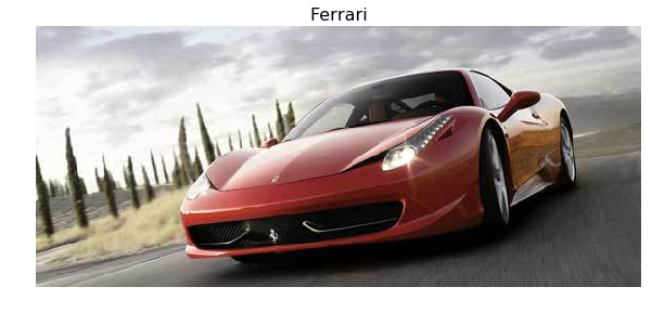
For this task I used the Stanford Cars Dataset. The data is a collection of images of cars and details about their make, model, and year. For the time being, I am not concerned about the model or year of the cars. I only want to build a model that predicts the make of the car based on the image (BMW, Audi…etc.). I downloaded the training set from here and the labels here. I then edited the labels of the images to only contain the make of the car, but exclude the model and year. Here is an example of an image from the training set and its label:
The training set consists of 8,144 images that belong to 49 different classes (car makes). I used 20 percent of the training set images to use as a validation set. The validation set should tell us how well the model is performing on previously unseen images. I resized all images to 224x224. The images have to be square to be able to use graphical processing units (GPUs) for accelerated computations. I chose the image size as balance between being large enough for the model to learn properly but small enough to reduce computational cost.
Preparing the Model
The problem at hand is a multi-class image recognition problem. To solve it, we need a model that is suitable for computer vision. In recent years, convolutional neural networks (CNNs) have been demonstrated to be the best models for computer vision. Experiments also showed that deeper (more hidden layers) models tend to achieve greater accuracy on complicated tasks in computer vision. However, increasing the depths of CNNs often leads to difficulties in model training. More recently, a variant of CNNs, known as Residual Networks (ResNets), were proposed to avoid the depth-related problems of normal CNNs. ResNets have since achieved state-of-the-art results in major image recognition tasks. For these reasons, I decided to use ResNet-50, a 50-layer ResNet model that can be used for image recognition.
Model Training
For the remaining sections we will proceed to train the model on the training data using various methods. Unless otherwise specified, all model training was carried out using the default settings of the fastai library, which will be discussed in this sections.
Prior to training, the final fully connected layers of the original pre-trained model are removed. The output from the final convolutional layer (a MaxPool layer) is fed into a batch normalization layer with Pytorch’s default parameters (epsilon=1e-05, momentum=0.1, affine=True). The output from batch normalization is then fed into a dropout layer with a keep probability of 0.25.
This is then fed into a fully connected layer containing 512 hidden units (neurons). Each unit applies the ReLU activation function. The output then goes through batch normalization and drop out as previously described, but the keep probability for dropout is 0.5. Finally the values are fed to a final output layer containing neurons that are equal to the number of class labels (i.e. 49 units). Each unit applies the logSoftMax function. The weights of the fully connected layers were initialized using the normal He initialization method.
The parameters of the model were updated using stochastic gradient descent with momentum. The momentum parameter was set to 0.9.
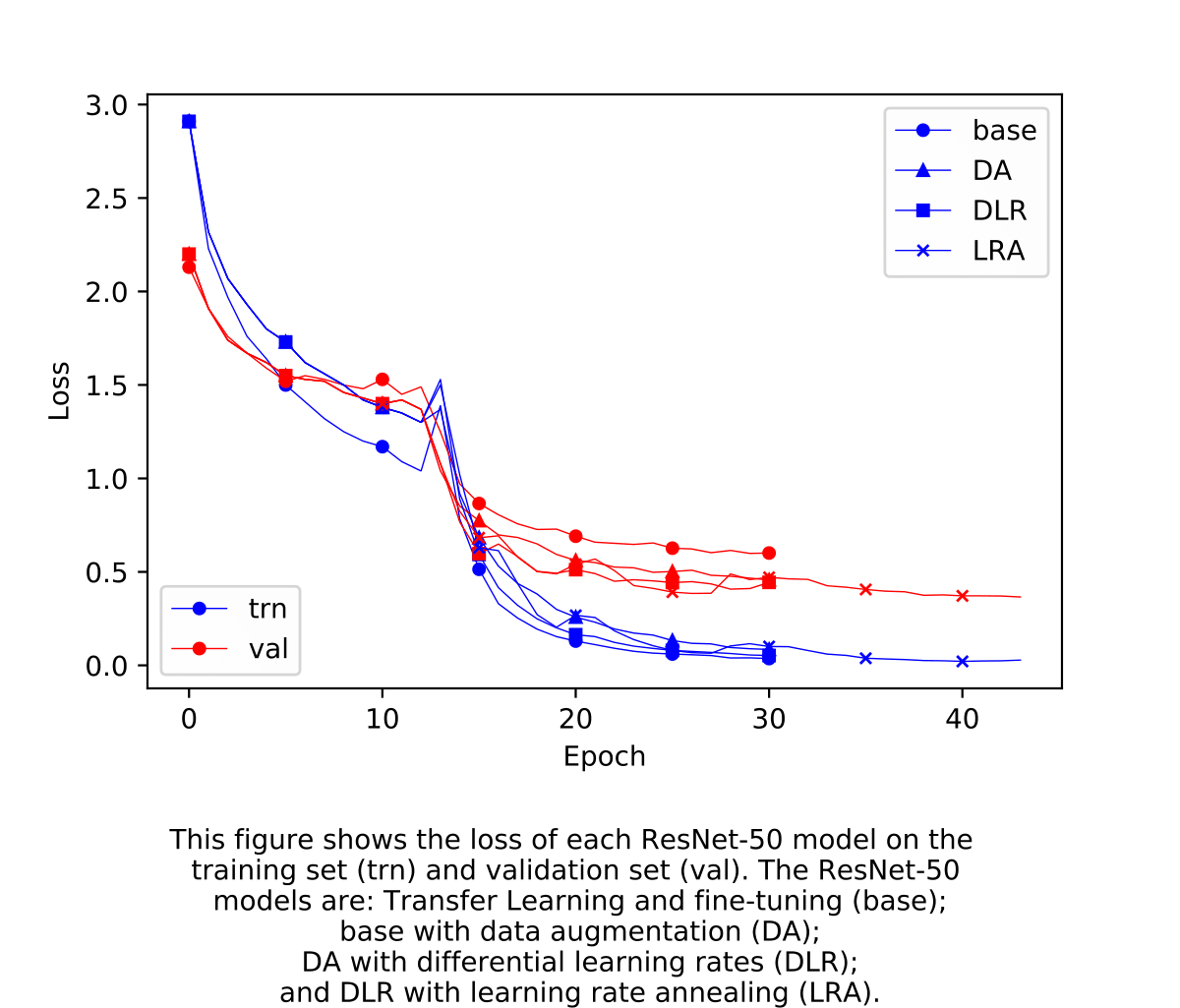
In the following sections, details of each experiment are discussed. The general aim of each experiment was to improve the model’s accuracy on the validation set. The first experiments use transfer learning and model fine-tuning; the second incorporates data augmentation; the third incorporates differential learning rates; and the final incorporates learning rate annealing during model training.
Transfer Learning
A common first step for training a deep learning model is to initialize the values of its parameters - the weights and biases. Our task represents a relatively complicated problem: the model has to be able to tell apart the different brands of cars, even though they all look rather similar to each other. In addition, our training set has a limited size of 8,144 images, which would make it difficult to train a model from scratch. For these reasons, we will use a pre-trained ResNet-50 model. This means that the model’s parameters will be initialized using the paramters of a ResNet-50 model that was trained on another image recognition task. This type of initialization is called Transfer Learning. Our ResNet-50 model has been pre-trained on ImageNet - a corpus of almost 14 million images.
As a start, I added a fully connected layer to the end of ResNet-50 and trained it on the raw data. In order to find a suitable learning rate, I used a method proposed by Leslie et al. [3]. It involves exponentially increasing the learning rate as the model trains on iterations until divergence occurs. This learning rate finding method is implemented in the fastai library. The plot generated below indicated that 0.08 would be a suitable learning rate.
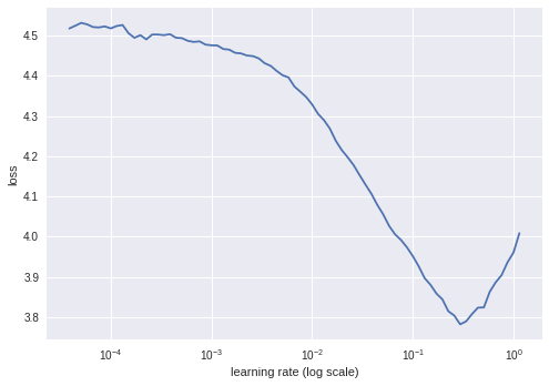
I then ran training for 13 epochs and achieved an accuracy of 57.2% on the validation set.
Model Tuning
Clearly, an accuracy of 57% is not very good. It is actually almost as bad as I am at recognizing cars. It is important to note that the parameters of the model’s hidden layers are optimized for recognizing the most common human-generated images. They are not optimized for solving our problem: recognizing cars. Therefore, I tried to fine-tune the model parameters by training again but this time allowing the hidden layer parameters to be updated during training. I first ran the learning rate method to find a suitable learning rate for fine-tuning. The plot below indicates that 0.001 would a suitable learning rate.
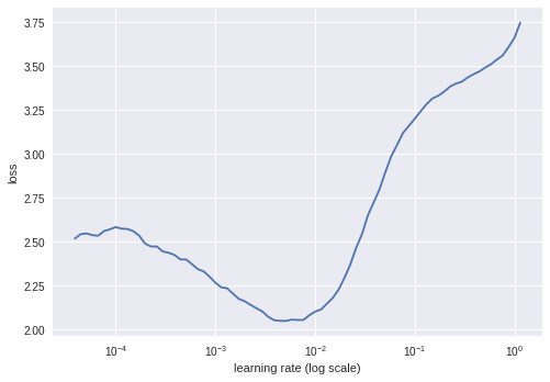
I then ran training for 18 epochs and achieved an accuracy of 83.3% on the validation set. Not too bad!
Data Augmentation
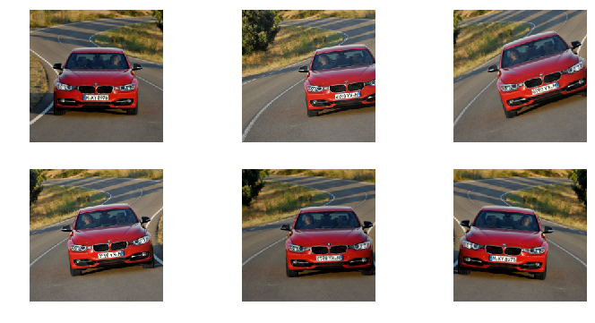
An 83% accuracy is much better, and the model became relatively good at recognizing the make of a car from its image. But can we do better? The data that we use for training has a limited size of 6,515 images without the validation set. We need the validation set in order to measure the performance of our models. However we can increase the size of our data using augmentation. Data augmentation basically involves creating edited versions of our images and adding them to our data. These edits include flipping, rotations and zooming in. For each image, we generate 5 random augmented images and add them to our data. Here is an example of a training image and it’s augmentations:
After data augmentation, we used the original pre-trained ResNet-50 for transfer learning (13 epochs), followed by fine-tuning (18 epochs). The model achieved an accuracy of 87.5%.
Differential Learning Rates
The parameters in the hidden layers of the pretrained ResNet-50 has learned image features at various levels of abstractions. The early layers learned high-level abstract features such as edges, while the final layers learned low-level features that are more specific to the image recognition task it was trained on. For these reasons, I wanted to study the effect of applying different learning rates for the different layers in the model. The basic logic is to use low learning rates on early layers, since they already learned the high-level features present in common human-generated images, but use higher rates for the final layers to better learn the specific features of our data. I specified three learning rates (0.001, 0.003, 0.01) for the model’s early, middle, and final layers, respectively. I then trained the original ResNet-50 model as previously described. The model achieved an accuracy of 88.8%.
Cyclic Learning Rate Annealing
To further improve the model, I added learning rate annealing to the training procedure. Learning rate annealing is a method that was recently proposed to improve training deep learning models. It basically involves reducing the learning rate throughout the iterations of an epoc. The learning rate is then reset for the next epoch, and so on. The annealing method applies a cosine functional form to reduce the learning rate during the iterations.
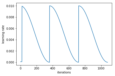
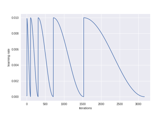
Furthermore, I added a multiplicative factor of 2 to the annealing method. This means that the annealing covers one epoch before it is reset, then two epochs before it is reset, and so on. Here is a plot of the learning rate during iterations of model training as an illustration
The model was trained using the original ResNet-50 model as previously described with annealing added during fine-tuning. This model achieved an accuracy of 89.9% on the validation set.
Test-time Augmentation
Earlier in this project, we used data augmentation on the training set to improve the model’s accuracy. Given a test image, what if we perform the same augmentations on it before predicting? This is called test-time augmentation. After training the model as previously described, I used TTA to predict on the validation set. The model achieved an accuracy of 92%.
Model Inference
After training our models as previously described. It is now time to measure their true accuracy on the test set. The test set consists of 8,141 images that were never used during any step of model training. The test set accuracy is a measure of the model’s ability to generalize what it learned during training to real-life applications. I saved all the models that we previously trained and computed their accuracy on the test set.
| Model | Val Accuracy (%) | Test Accuracy (%) |
|---|---|---|
| Transfer Learning | 57.2 | 57.4 |
| Fine-tuning | 83.3 | 82.5 |
| Data Augmentation | 87.5 | 85.9 |
| Differential Learning Rates | 88.8 | 88.1 |
| Learning Rate Annealing | 89.9 | 89.9 |
| Test-time Augmentation | 92 | 91 |
The Ultimate Test (JUST FOR FUN)
After all this work, I wanted to put the final model to the test. How good is it actually at recognizing the make of a car from its image? Let’s find out! I started looking for images on Google of cars that I like. Here is the first one:
I performed the same transformations on it as I did with the training data. I then gave it as input to the model and waited to hear its prediction. And…
Computer Says: …Tesla!!!
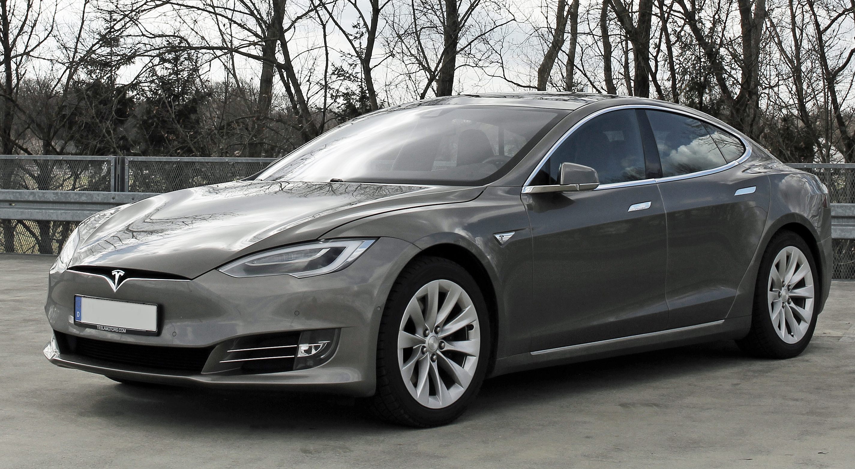
I also repeated it with this image:

And Computer Says: …Mercedes-Benz!!!
I find it interesting that both images had cars with model and year that was not in the training data. But despite of this the model was able to correctly predict the make of the cars!
How cool is this?! That’s deep learning for you.
References
[1] Stanford Cars Dataset: https://ai.stanford.edu/~jkrause/cars/car_dataset.html
3D Object Representations for Fine-Grained Categorization Jonathan Krause, Michael Stark, Jia Deng, Li Fei-Fei 4th IEEE Workshop on 3D Representation and Recognition, at ICCV 2013 (3dRR-13). Sydney, Australia. Dec. 8, 2013.
[2] fastai library: https://github.com/fastai/fastai
[3] Learning rate finder: Cyclical Learning Rates for Training Neural Networks.
Leslie N. Smith U.S. Naval Research Laboratory, Code 5514 4555 Overlook Ave., SW., Washington, D.C. 20375