Summary

This post explains the GELU activation function, which has been recently used in Google AI’s BERT and OpenAI’s GPT models. Both of these models have acheived state-of-the-art results in various NLP tasks. For the busy readers, this section covers the definition and implementation of the GELU activation. The rest of the post provides an introduction and discusses some intuition behind GELU.

Definition

GELU was proposed in this paper, which defines the function as:

where $x$ is an input value, \( X \) is a Gaussian random variable with zero-mean and unit-variance that models the input, and \( P(X \leq x) \) is the probability that the input can be less than or equal to the given value.

Implementation

GELU can be computed using the Gauss Error function, which is implemented in many numerical libraries such as SciPy, TensorFlow, and PyTorch, as such:

where \( erf(.) \) is the Gauss Error Function. Here are example implementations of GELU using three common numerical libraries in Python:

#Using TensorFlow
import tensorflow as tf
def gelu(x):
    cdf = 0.5 * (1.0 + tf.erf(x / tf.sqrt(2.0)))
    return x * cdf

#Using PyTorch
import torch
def gelu(x):
    cdf = 0.5 * (1.0 + torch.erf(x / np.sqrt(2.0)))
    return x * cdf

#Using SciPy
from scipy.specials import erf
def gelu(x):
    cdf = 0.5 * (1.0 + erf(x / np.sqrt(2.0)))
    return x * cdf

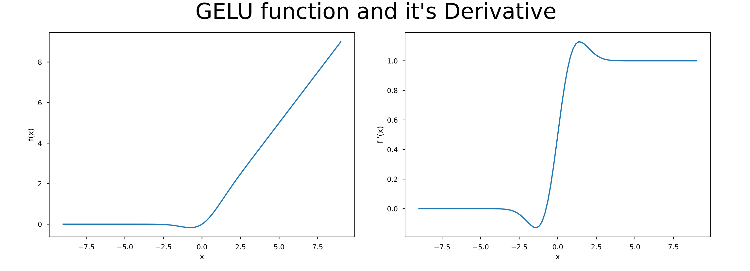
And here are visualizations of the GELU activation and it’s derivative:

Note: Project code can be accessed here: https://github.com/AlTheEngineer/Deep-Learning-Fundamentals

Intuition

The authors that proposed GELU argue that it is a deterministic non-linearity that encapsulates a stochastic regularization effect. In the following, we’ll discuss the detailed intuition behind GELU so that the reader can independently assess the author’s argument.

Before we begin, recall that the ReLU activation is simply an identity mapping for positive inputs and a zero mapping otherwise (zero-or-identity mapping). Now, let’s describe a stochastic zero-or-identity mapping from which the GELU can be derived. Assume that the input \( X \) is such that

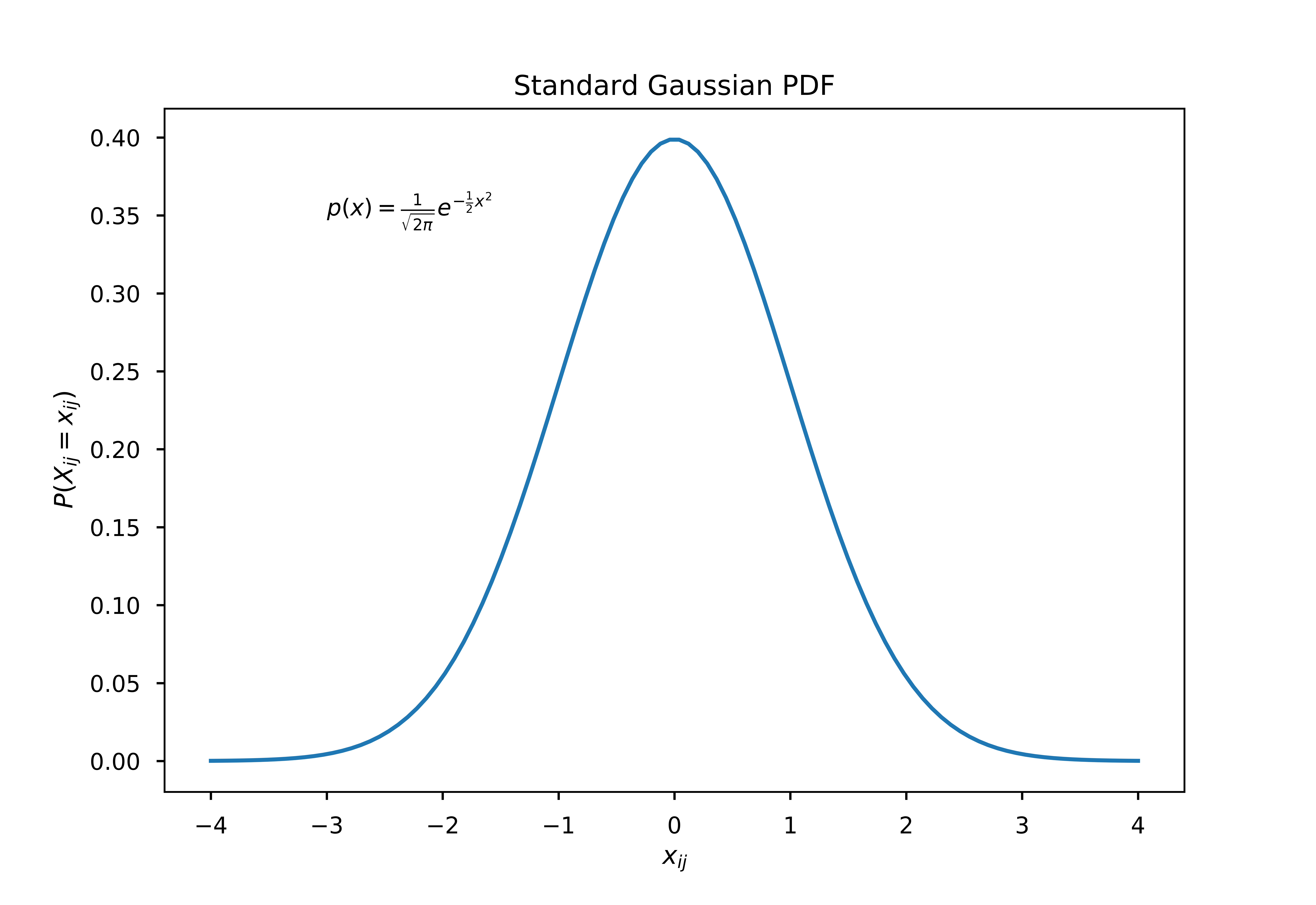
where \( m \) is batch size and \( n \) number of input features. This essentially means that we assume that each input feature is a random variable of the normal distribution with a mean of zero and a standard deviation of one. This can be visualized using the probability density function (pdf) of the distribution, as such:

We now want to apply a zero-or-identity mapping to \( X_{ij} \), similar to ReLU but in a stochastic (random) way. We would also like larger values of \( X_{ij} \) to have a higher probability of being perserved (i.e. not being dropped). We can do this by using by defining the following:

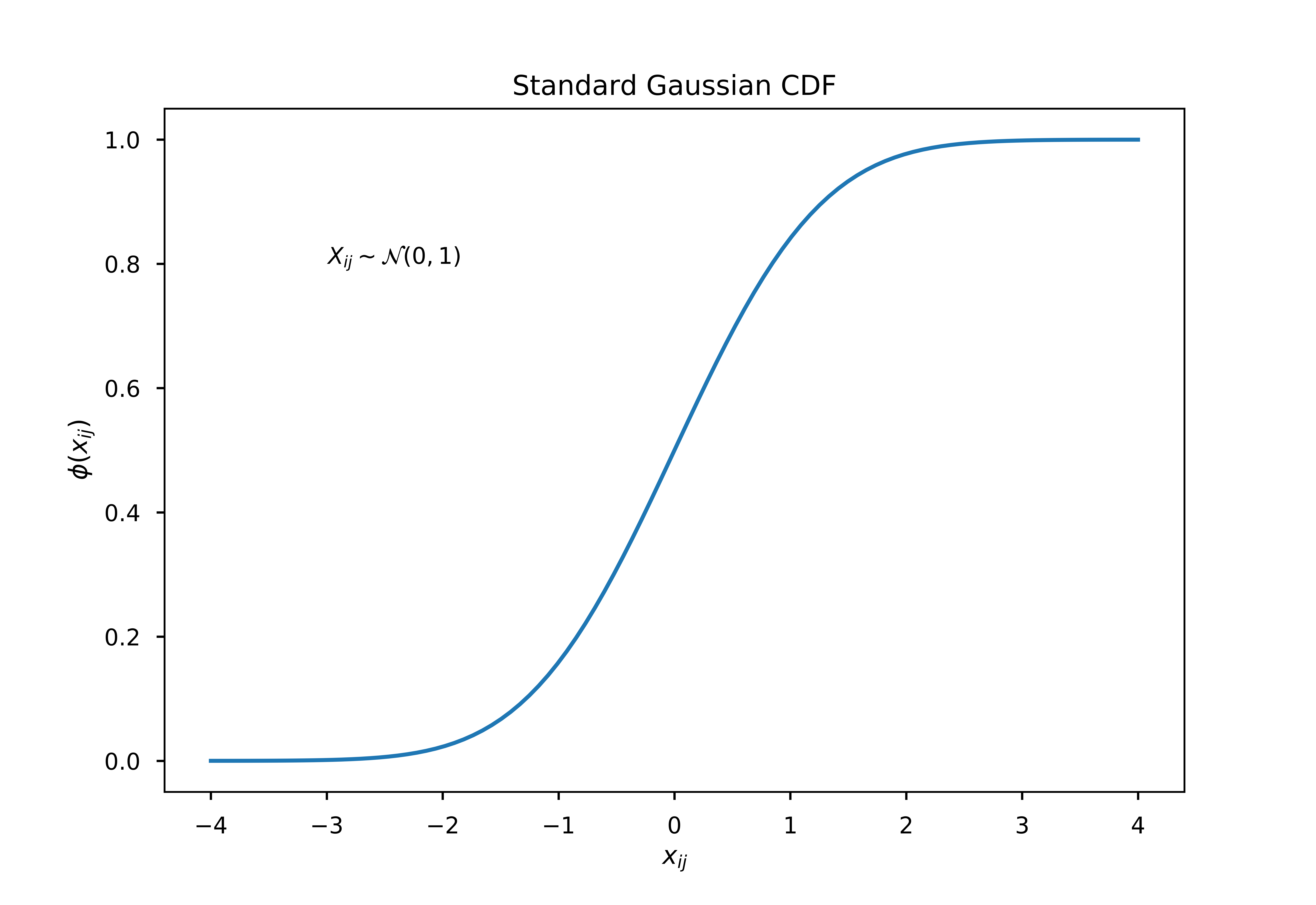
This essentially means that a specific input value \( x_{ij} \) gets preserved with probability equal to the probability that any input \( X_{ij} \) is either less than or equal to it. For discrete probability distributions, this can computed simply by summing up the probabilities of all the values less than or equal to \( x_{ij} \). However for continuous distributions like the Gaussian distribution, we compute this function using integration:

where \( \phi(x_{ij}) \) is known as the cumulative distribution function (cdf) and is shown in the figure below:

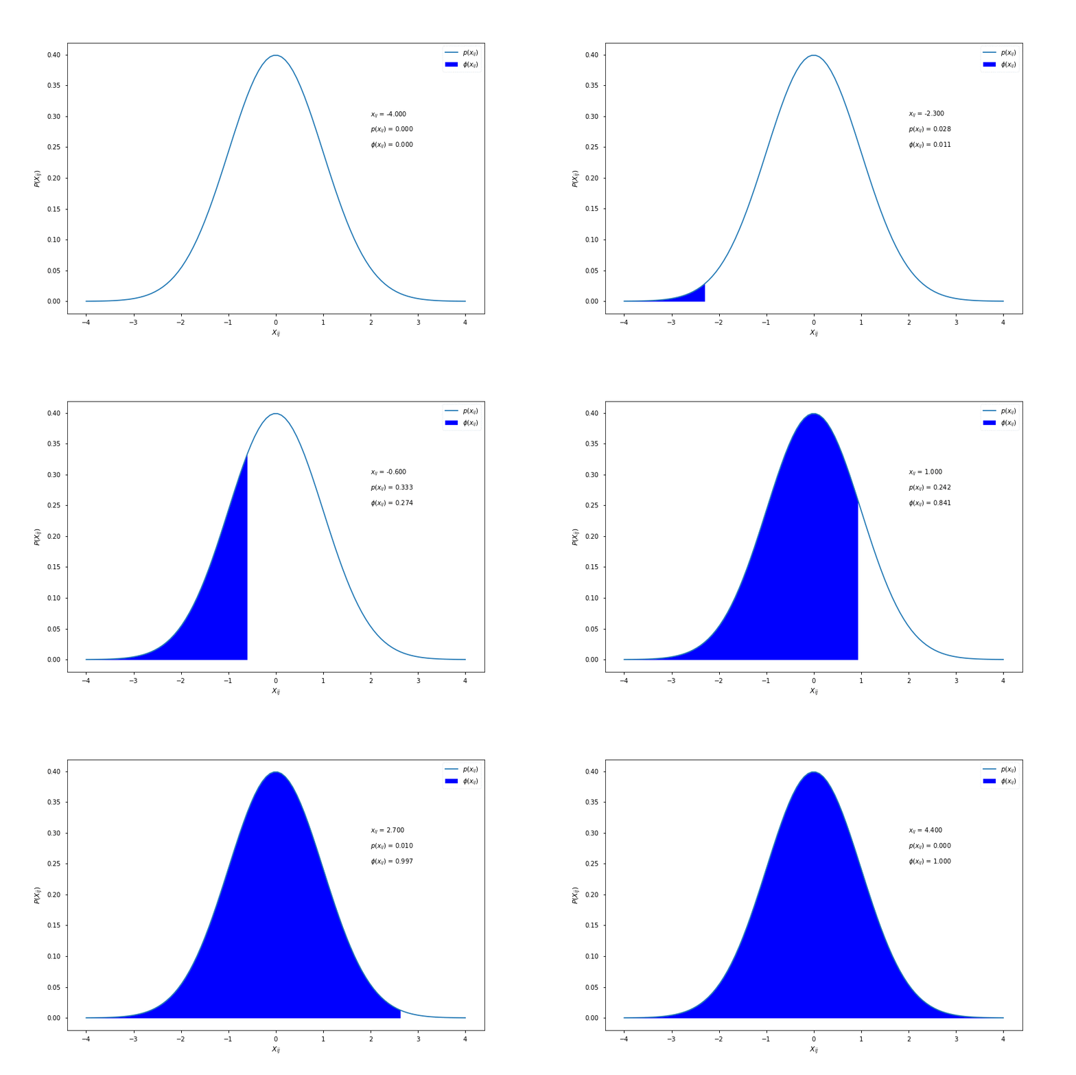
As a conceptual aid, \( \phi(x_{ij}) \) is equal to the area under the pdf curve to the left of \( x_{ij} \). Here is a visualisation for different values of \( x_{ij} \):

Computing \( \phi(x) \)

The Gauss Error function (erf) is a special function that occurs in probability, statistics, and partial differential equations. The erf is defined as

There are various algorithms to approximate erf and it is implemented in many libraries such as SciPy, TensorFlow, and PyTorch. Therefore, we would like to compute \( \phi(x) \) using erf. In the following, we will use algebraic manipulations to express \( \phi(x) \) in terms of \( erf(x) \).

Let \( t=\frac{z}{\sqrt{2}} \), so we can re-write erf as:

Now, let’s split this integral into two parts by changing the limits of integration, like this:

Now, take a moment and look at the equation for \( \phi(x) \) that we defined above. Notice the resemblence? Yes, that’s right:

Now, take a look at the figure above that visualizes \( \phi(x) \) in terms of the area under curve. Can you tell what \( \phi(0) \) would be? Yeah exactly, it’s half.

But we wanted \( \phi(x) \) in terms of \( erf(x) \), not the opposite! Well, we can simply do that by letting \( y = \frac{x}{\sqrt{2}} \), so that:

And voila!

Creating A Deterministic function

What we have done so far is define a stochastic regularizer that applies a zero-or-identity (SOI) mapping to the input \( x \) with probability \( \phi(x) \). Now we would like to use this to create a deterministic function to be used as an activation. Notice that the SOI can do one of two things: apply an identity mapping with probability \( \phi(x) \) or a zero mapping with probability \( 1-\phi(x) \). This corresponds to a Bernoulli trial. The expectation (mean value) of this trial is:

And this is exactly what the GELU activation function is!

Computing the Derivative

Training deep learning models relies on the backpropagation of error gradients throughout the network’s parameters. Therefore, we need to be able to compute the derivative of GELU with respect to the input. Here is that derivative:

where \( P(X=x) \) is the value of the pdf at \( x \).